Safety-Stock Calculations Are Risky – Demand, Lead Time and Service Level

This is a big and touchy topic, I know. I intend only to begin a dialog, not present an exhaustive treatise. First, let me define what I mean by “safety stock,” or SS: Not the restrictive, MRP-specific adder to gross requirements, but the general concept of buffer inventory. SS, determined correctly and optimally, protects against random variations in demand and supply, up to a desired fill rate.

Paypal

Help us to keep bringing you this high-quality content. Please donate today!

Also, forgive my use of the term “optimal,” now unfortunately a hackneyed buzzword. In its true sense, optimal SS enables any inventory item in any location to achieve – but not needlessly over-achieve – its target service level with the minimum on-hand quantity, consistently and without expediting, taking into account the item’s current supply-chain parameters. Really, the ability to determine truly optimal SS, and thus optimal inventory levels, is fundamental to operational excellence.

At first glance, optimal SS seems simple, with just 3 obvious variables:

1. Target service level(SL), such as a 99% fill rate
2. Demand (D) random variation, as measured by perhaps standard deviation
3. Lead time (LT) random variation, also as measured by perhaps standard deviation

Plenty of algorithms use these variables. You likely have some version of a SS calculation in a spreadsheet. Does it work for you? Are you sure it is optimal for you? In the interest of operational excellence, the ideal technique for determining optimal SS, and thus optimal inventory, is one that is correct, comprehensive, fact- and data-driven, and objective. By contrast, if your definition of ideal is simply that it be spreadsheet-friendly, this article has little to offer you. That said, I’m confident I can show you a better inventory/SL position than what you have currently. (I want that to sound inviting, not challenging!)

SS=z*√(((Mean LT*(Stdev of D^2))+((Mean D^2)*(Stdev of LT^2))), or variations on it, is a popular calculation encompassing the 3 obvious variables. Next, a partial list of common real-world factors not in this formula:

1. Mean and standard deviation are the two parameters defining a normal distribution. Yet it’s almost guaranteed that none of your items’ actual D patterns are well fit by a normal distribution – likely, not even close. D intermittency alone (and most of your items have intermittency) makes normal a bad fit. D cannot be less than zero, but normal distributions can and do include negatives. Normal-based math and stats are unlikely to get you “close enough.”
2. Likewise, a normal distribution isn’t likely a good fit for LT. It cannot be less than 1 (of whatever time unit of measure you use), but it has no practical upper bound. LT is typically either right-skewed or multi-modal. Normal-based calculations are unreliable at a minimum, and can even be dangerous.
3. Your actual SL is a quantity-based fill rate (number of units, lines, orders, etc.), but a simple “z” multiplier represents the probability of no stockout events. Your stockout quantity affected is important – a big stockout is more painful than a small one. By contrast, z assumes each stockout is the same pain, no matter how small. Mathematically, z overstates the required SS. (And if you use NORMSINV to derive z, it again wrongly assumes a normal distribution.) Certainly, you can use a unit-normal-loss z multiplier, but this greatly complicates the calculation and the required input data. (And yet again assumes a normal distribution.)
4. Your customers are sensitive not only to SL, but also to its consistency. No customer is happy if you achieve target SL just one month (or week, quarter, etc.) out of two. This concept is called confidence, and it’s different than SL. Formulas ignore this important factor, and it’s extremely challenging to make a deterministic algorithm accommodate confidence.
5. SL cycle, the time period during which you measure actual SL, is important. Common sense says that typically you require more inventory to achieve a consistent monthly SL than a daily one. Formulas, however, exclude SL cycle. (Technically, they assume it to be the same as LT.)
6. Real-world past-due D backlog often carries over, making other D late. You know it’s true, but the formula assumes D not fulfilled on time is always canceled.
7. MOQ (along with order multiple) or similar reorder-quantity constraints. Larger MOQs, though undesirable because they increase cycle stock, also drive longer replenishment cycles (RCs). Longer RCs provide de facto SS, since a stockout may be virtually impossible for so many days or weeks after the receipt of a large MOQ. Likewise, small MOQs (or EOQs) drive frequent receipts. Frequent inbound receipts also provide de facto SS. In any case, MOQ reduces the incremental quantity of formal SS. Most formulas don’t do this; those that attempt it are incorrect.
8. Similar to MOQ, fixed replenishment-review intervals provide a degree of de facto SS, also reducing the quantity of formal incremental SS. Formulas ignore this common but important interval. (Technically, they assume replenishment is reviewed continually).
9. Replenishment method affects both optimal SS and the inventory parameters that achieve it. For example, classic ROP may require more SS, but lower quantity on hand, than does “two-bin” kanban. And certainly, classic ROP’s defining parameter is ROP, whereas two-bin kanban’s parameter is quantity per bin. The ability to accommodate replenishment method, and then translate SS into the appropriate associated parameter(s), is beyond the capability of common SS calculations.

This, of course, is not an exhaustive list. Now, let’s take a deeper dive into the first three factors above.

FACTOR 1: Demand for your items is not best represented by a normal distribution. Yet the calculation uses the two parameters – mean and standard deviation — defining a normal distribution. D intermittency alone (and most of your items have intermittency) makes normal a bad fit. D cannot be less than zero, yet normal distributions can and do include negatives.

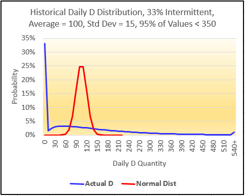
But let’s be practical: Do normal-based math and stats get you “close enough”? The chart below shows an item with a 33% intermittency (D = zero for 1 day out of 3) and a mild 0.15 coefficient of variation (CV). The right tail of actual demand (blue line) extends far beyond (12% of actual demand data points!) that of the normal distribution (red line). The right tail presents the biggest risk to SL, and a normal distribution leaves that risk exposed!

FACTOR 2: A normal distribution isn’t likely a good fit for LT. LT cannot be less than 1 (of whatever time unit of measure you use), but it has no practical upper bound. LT is typically either right-skewed or multi-modal (supplier A vs. supplier B, etc.).

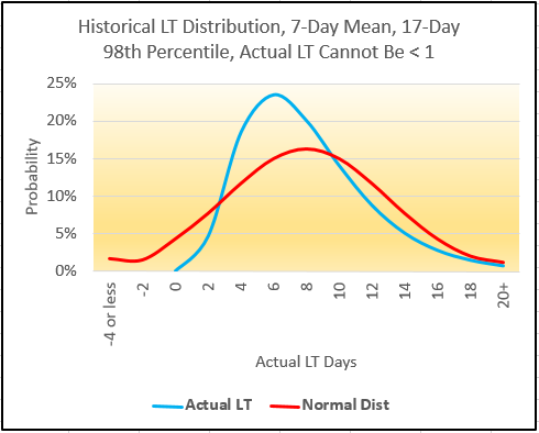
Again, let’s be practical: Does this present a real, significant risk? Let’s say that an item’s average LT is 7 days, and 98% of the time LT is 17 days or less. Given these parameters, a normal distribution “thinks” that about 11% of actual LTs are < 1 day, and that about 8% are < zero! See chart below.

When LT CV exceeds about 0.3, a normal distribution assumes actual LTs of less than 1, and even less than 0. Likewise, when your actual LTs are multi-modal – which isn’t unusual – normal is a bad assumption. For LT, normal-based calculations are risky.

FACTOR 3: The z multiplier represents the probability of no stockout events. Your actual SL is a quantity-based fill rate (number of units, lines, orders, etc.). To you and your customer, a big stockout is more painful than a small one. By contrast, z assumes each stockout is the same pain, even if the short quantity = 1.

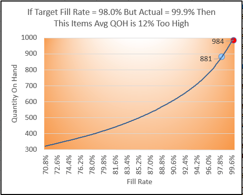
Once more, let’s be practical: Does this result in a meaningful difference? For an item with considerable demand quantity, say 1000 in a month, a stockout of 1 causes a 99.9% fill rate. However, the z multiplier considers this to be 1 stockout in 30 days, and thus 29 days out of 30 days = a 96.7% probability of no stockouts.

Using the Excel NORMSINV function on 96.7% yields z multiplier = 1.83. If your target SL is, say 98.0%, the z multiplier thinks you failed. In fact, though, your quantity-based actual fill rate was 99.9%. So Yes, there is a meaningful fill-rate difference. But is there a meaningful inventory difference? See chart below. In this example, the z multiplier alone drives an actual 99.9% fill rate against a target of 98.0%, resulting in 12% more inventory than the optimal level.

If this item’s fill rate was 99.9% for, say 12 months – against a target SL of 98.0% — you would likely conclude that it has too much SS. Mathematically, z overstates the required SS. (And if you use NORMSINV to derive z, it again wrongly assumes a normal distribution.)

In following articles, I’ll go into more detail on 6 more critical factors that supply-chain professionals intuitively know have an effect on optimal SS and thus optimal inventory levels – and these are entirely missing from the popular SS calculations.

I’ll also give you a sneak preview of what I propose as a solution to the failings that are inherent in an inventory-optimization calculation: A simulation that correctly and comprehensively addresses all relevant real-world factors affecting optimal inventory, reliably-achieved target service levels and no expediting.

Of course, a spreadsheet provides neither the capacity nor the speed for a simulation that your organization can depend on. However, my recommendation is this – build a simulation that represents your unique combination of relevant factors. It will help you immensely in understanding the data you will need to gather in order to use a correct, comprehensive, fast and commercially-available Monte-Carlo-style inventory simulation.

I trust you will find this post to be a springboard for discussion among my esteemed operational-excellence peers!

David McPhetridge

David has over 30 years of experience in lean and flow, MRP, information technology, cost accounting and finance across a broad range of industries. Since 1994, he has implemented lean and flow worldwide in scores of facilities and industries, including regulated environments.

David holds two patents involving optimal inventory, and is the inventor of the analytical technology and methodology behind Right Sized Inventory LLC’s comprehensive inventory-optimization solution.

David has implemented multiple MRP/ERP systems, and has led, driven and developed many post-implementation MRP/ERP enhancements. He has managed cost accounting in both work-order and repetitive-manufacturing environments, and has been Director of Finance in a division of Emerson Electric.

Connect with David on LinkedIn   |   View the Right Sized Inventory page on LinkedIn