Should Safety Stock Include Demand Forecast Error?

Yes, I’m broaching a hot topic. This article is deliberately not exhaustive, leaving plenty of room for further discussion. My intent: to encourage constructive, informative conversation among my many LinkedIn supply-chain experts. I have done my best to ensure that I have supported all my assertions with facts, analysis and calculations.

Paypal

Help us to keep bringing you this high-quality content. Please donate today!

Here is my theme: Forecast-to-actual demand variation has no place in determining safety stock (or buffer inventory of any form). Regarding actual demand, safety stock applies only to common-cause variation. Please follow my line of reasoning, and I so appreciate your interest, attention and participation in a discussion!

First, three definitions:

1. Safety stock, or SS: Not just the MRP-specific adder to gross requirements, but the general concept of buffer inventory. SS protects against common-cause random variationsin demand and supply to achieve a target fill rate consistently, without expediting.

2. Forecast bias (uniform): Chronic, ongoing multi-period bias with a uniform, same-direction difference between actual-demand and forecast-value averages for those periods. In this scenario, we will not include common-cause variation.

3. This special case of non-uniform forecast bias, focused on: inaccurately-predicted timing, magnitude, behavior of special causes. Whereas a biased forecast (above) has a different average than that of actual demand, this special case has the same  In this scenario, we will not include common-cause variation.

Next, the most basic causes of demand forecast error, or DFE: Not to oversimplify a very complex subject, but DFE results from one or more of these 3 scenarios:

1. Actual demand common-cause variation (no forecast bias)
2. Forecast bias, uniform (see above)
3. Inaccurately-predicted timing, magnitude, behavior of special causes, a special case of non-uniform forecast bias(see above)

Now, these DFE scenarios in more detail:

• Scenario 1 – DFE from common-cause variation in actual demand:– The forecast correctlypredicts timing, duration, magnitude and behavior of special causes with no chronic bias. (Or, lacking special causes, correctly predicts average actual demand. I’ll focus on forecasts with systematic special causes – using trend as an example).
  – No forecast can predict a specific value for common-cause variation in a period – by definition, common-cause variation has unpredictable timing. The purpose of SS is to addressactual common-cause variation in both demand and supply. The easiest way to do this, with the least undesired distortion, is to analyze historical demand directly, rather than DFE and its inherent non-common-cause distortions.
• Scenario 2 – DFE from forecast bias (uniform, see above):-When mean forecast demand is chronically and consistently above or below mean actual demand. Its cause? Perhaps over- or under-optimism, unmaintained planning BOMs and other culprits. Bias is not common-cause demand variation and has no place in determining SS.

• Scenario 3 – DFE from (non-uniform) inaccurately-predicted timing, magnitude and behavior of special causes,-such as the effects of trend, seasonality, promotions, introductions and phase-outs. Of course, sales/marketing’s ability to predict such special causes is critically important. This minimizes the inclination to increase SS as protection against forecast error. Technically, this scenario involves bias, but in our example, forecast and actual averages match in total for all periods.

These three scenarios rarely exist alone. Instead, DFE consists of their combined influence. My examples have isolated each cause to illustrate its effect on SS. Supply-chain professionals – consider these practical questions:

• Is it realistic – for each and every inventory item in each and every location – to isolate the common-cause component of DFE?
• Since SS applies only to common-cause variation in historical actual demand, why not simply analyze this actual demand, avoiding the extra effort, and risks of diluting common-cause variation, inherent in determining and using DFE?

Our discussion uses the basic replenishment logic shown below. Demand may be from forecast, actual or a combination, depending on any stocked item-location’s specific replenishment method:

Replenishment Qty = Demand + SS – (QOH + On-Order)

I will use this common heuristic for calculating DFE-based SS,

SS = z * z factor * √ lead time in forecast periods * MAD

In which:

• The z variable (typically generated using Excel’s NORMSINV function) converts a target probability of no stockouts(service level, or SL) to a multiplier.
• The z factor, 1.2533 or √(π / 2), enables z to be applied to MAD instead of to standard deviation.
• The square root of lead time(LT), expressed in forecast periods, enables the result to reflect variation during LT. Note: in the examples below, 1 LT = 1 forecast period.
• MAD, mean absolute deviation, quantifies the difference between forecast and actual.

I am not proposing that this SS heuristic is the right one, using it instead only as a recognized common calculation for comparison. Now, for the three basic DFE-cause scenarios:

Scenario 1: Safety Stock for DFE from Common-Cause (Random) Variation in Actual Demand

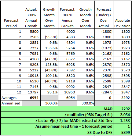
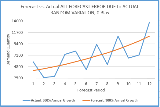
This scenario represents the type of variation for which SS is intended. See this scenario’s data in the table and chart below:

• Forecast: 300% annual growth (9.6% month-over-month), mean = 6954
• Actual (same time frame): 300% annual growth, mean = 6954
• Scenario conclusion: Forecastcorrectly predicted timing and magnitude of trend. Forecast has no chronic bias. All forecast-to-actual variation is due to actual demand common-cause variation.
• With common-cause variation as the primary component of DFE, DFE-Based SS = 5899

Next, let’s construct a month-by-month perpetual inventory using this forecast-to-actual data. See tables and chart below:

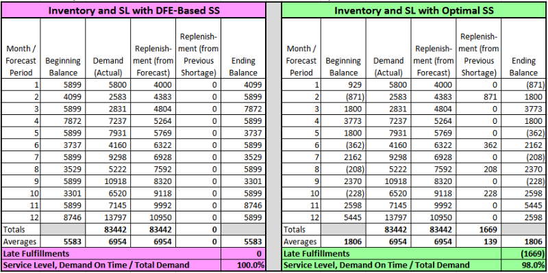
Left table above: inventory and SL performance using the DFE-based SS quantity. The right table above has been optimized to achieve the desired 98% SL. DFE-based SS drives inventory too high, achieving an undesired 100% SL and average quantity on hand, AQOH, that’s 3.1 times higher than optimal.

Here is how the perpetual-inventory tables above work, along with all to follow:

• Initial Beginning Balance =SS only(whether DFE-based or optimal)
• In a month, all Replenishments are received before they cause a late fulfillment, so long as Demand does not exceed Receipts + Beginning Balance
• In a month, lateness (negative inventory balance) occurs only to the extent that Demand exceeds Receipts + Beginning Balance
• All Demand is actual, not forecast
• Replenishments are the total of:
  – Forecast demand and
  – Negative prior-month Ending Balance (i.e., negative current-month Beginning Balance)

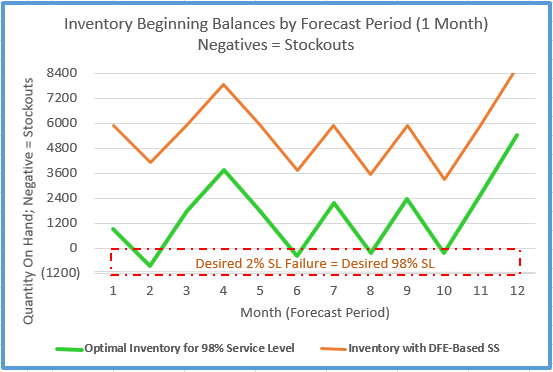
Next, the chart below considers inventory Beginning Balances by Month/Forecast Period when all DFE is due to common-cause demand variation. Negative balances indicate stockouts. We see that for this scenario, DFE-based SS is not optimal, resulting in more inventory than necessary.

(NOTE: These results also suggest that common, popular SS calculations such as the one we’re using are inherently flawed.)

Scenario 2: Safety Stock for DFE from Forecast Bias:

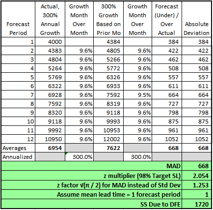
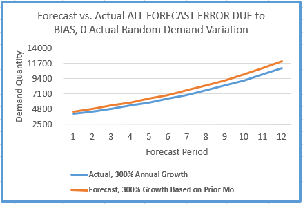
This scenario represents a type of forecast error for which SS is not intended. See the table and chart below for this scenario’s data:

• Forecast: 300% annual growth (9.6% month-over-month), mean = 7622
• Actual (same time frame): 300% annual growth, mean = 6954
• Scenario conclusion: Forecastcorrectly predicted growth trend rate. No common-cause demand variation. However, forecast, including multi-period mean, is constantly and consistently higher than actual. All forecast-to-actual deviation is due to forecast bias.
• With DFE’s dominant component as forecast bias,DFE-Based SS = 1720

Again, see tables and chart below for a month-by-month perpetual inventory using this forecast-to-actual data:

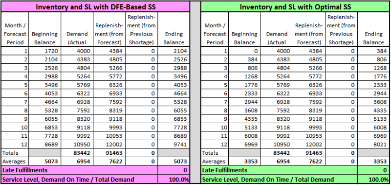
Left table above: inventory and SL performance using the DFE-based SS quantity. The right table could not be optimized to achieve the desired 98% SL.

Note – 98% SL is achievable, but only by employing negative SS (possible with ROP, but not with MRP). Chronic positive bias alone provides more than enough de facto SS, even when formal incremental SS = 0. DFE-based SS drives inventory even higher, achieving an undesired 100% SL and AQOH that’s at least 1.5 times higher than optimal.

Remember, an overview of how the tables above work is in Scenario 1.

Next, see chart below for this scenario’s inventory Beginning Balances by Month/Forecast Period: all DFE due to forecast bias. Note – this scenario has no stockouts. The chart highlights that for this scenario, forecast bias, DFE-based SS is not optimal, resulting in more inventory than is needed.

(NOTE: If using DFE-based SS, bias should be excluded, though this is often unreasonable in practice.)

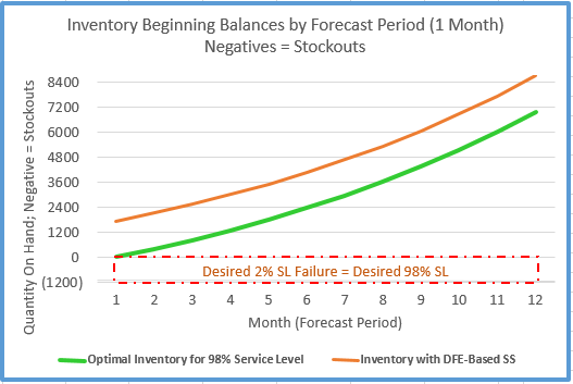
In practice, a supply-chain professional may not be able to check all of his or her inventory items for forecast bias. Yet bias distorts common-cause demand variation needed for DFE-based SS. Only historical actual demand data, not DFE, is meaningful for correct SS.

Scenario 3: Safety Stock for DFE from Inaccurately-Predicted Timing, Magnitude, Behavior of Special Causes

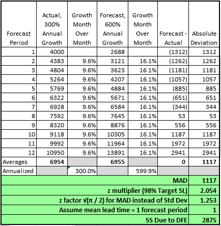
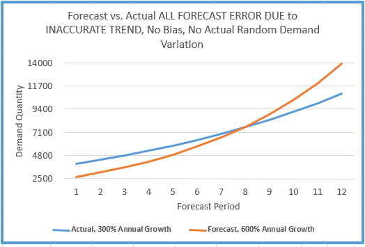
Once more, this scenario’s data, in the table and chart below, represents forecast error, for which SS is not intended:

• Forecast: 600% annual growth (16.1% month-over-month), mean = 6954
• Actual (same time frame): 300% annual growth, mean = 6954
• Scenario conclusion: Forecastincorrectly predicted timing and magnitude of trend. Forecast has no chronic bias (same mean as actual). Actual demand has no common-cause variation. All forecast-to-actual deviation is due to inaccurately-predicted timing, magnitude, behavior of special causes. DFE-Based SS = 2875

The tables and chart below show a month-by-month perpetual inventory using this forecast-to-actual data:

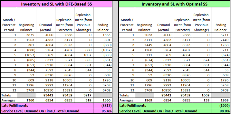
Left table above: inventory and SL performance using the DFE-based SS quantity. The right table above is optimized to achieve the desired 98% SL. The incorrectly-predicted timing, magnitude and behavior of special-cause trend results in insufficient inventory to support the 98% target SL. In this scenario, DFE-based SS causes inventory to be 31% lower than optimal, resulting in an undesired 95.4% SL and late fulfillments that are 2.3 times higher than desired.

Remember, Scenario 1 contains an overview of how the tables work.

Below, see this scenario’s inventory Beginning Balances by Month/Forecast Period, in which all DFE is due to incorrectly-predicted timing, magnitude and behavior of special-cause trend. Negative balances indicate stockouts. For this scenario, incorrectly-predicted special-cause trend, DFE-based SS is not optimal, resulting in less inventory than is needed.

(NOTE: Again, forecast error due to incorrectly-predicted systematic special-cause variation – such as trend – should be excluded from DFE-based SS. Easy to say; often unreasonable in practice.)

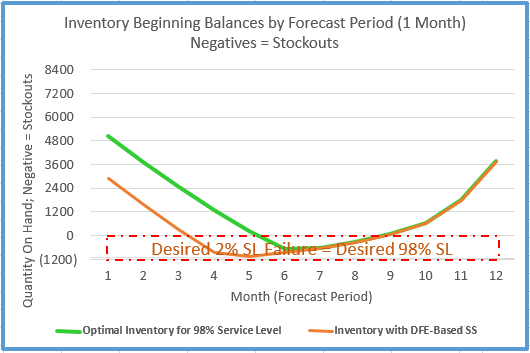
In a real-world setting, a supply-chain practitioner may not reasonably be able to check all of his or her inventory items for the effects of incorrectly-predicted systematic special-cause variation. Correct SS requires historical actual demand, not DFE, which often includes systematic variation.

Conclusions

In none of the three DFE scenarios, covering the spectrum of basic DFE causes, does DFE-based SS provide optimal inventory levels. It simply has no place in SS. But why? In summary:

• SS protects against common-cause random variations in actual demandand supply. Yet DFE is commonly tainted by other influences (such as in scenarios 2 and 3)
• Scenario 1, with solely common-cause demand variationand an unbiased forecast, shows that DFE is not the best demand-variation source for SS analysis. Instead, SS requires actual historical demand. (Note: the DFE-based SS formula used in this article is intended for just this scenario. One shortcoming of this formula – it assumes event-based service-level measurement, whereas in the real world, service level is a quantity-based fill rate)
• Scenarios 2 and 3 have no common-cause demand variation, but the forecastsincorrectly predict mean demand, providing forecast-to-actual deviation for which the DFE-based SS calculation is not intended
• What if historical actual demandcommon-cause variation doesn’t represent expected future behavior? What if we expect known special causes, such as trend, to continue – perhaps also existing in the historical actual demand? In order to determine truly optimal SS, we may need to pull out the systematic component of variation in the historical data. Then, as needed, apply statistically-sound techniques to predict expected future special-cause behavior. Removing demand variation’s systematic component spans the spectrum from easy to challenging, and is the topic of a future post.
• As for chronic, uniform/near-uniform forecast bias: Perhaps a supply-chain colleague will take on this question. In theory, S&OP minimizes bias, ensuring reasonable and realistic1) high-level forecast optimism or pessimism and 2) mix assumptions – planning BOMs, etc. In practice, this is an elusive challenge!

As we resolve this S&OP challenge effectively, we also reduce the concern about increasing SS to protect against forecast error. Instead, we appropriately base our SS analysis on historical actual demand, confidently using collaborative, S&OP-validated, forecasted special-cause demand variation (such as trend) as statistically-appropriate modifiers to the SS analysis as needed.

Finally, what of incorrectly-predicted timing, magnitude and behavior of special causes (with no chronic bias – as described at the beginning of this post)? As we just considered, a sales/marketing team that accurately forecasts such demand behavior is worth their weight in gold – an understatement even at USD 1,200 per ounce! In any case, accurately-predicted special causes enable us to focus a correct SS calculation on its true demand target: common-cause variation.

In reality, forecast error includes unavoidable risk that SS cannot mitigate, instead requiring deliberate, effective forecasting refinements and enhancements that all businesses need and pursue.

David McPhetridge

David has over 30 years of experience in lean and flow, MRP, information technology, cost accounting and finance across a broad range of industries. Since 1994, he has implemented lean and flow worldwide in scores of facilities and industries, including regulated environments.

David holds two patents involving optimal inventory, and is the inventor of the analytical technology and methodology behind Right Sized Inventory LLC’s comprehensive inventory-optimization solution.

David has implemented multiple MRP/ERP systems, and has led, driven and developed many post-implementation MRP/ERP enhancements. He has managed cost accounting in both work-order and repetitive-manufacturing environments, and has been Director of Finance in a division of Emerson Electric.